Monads in Programming

As Douglas Crockford once mentioned in his talk, once you understand the monads, you lose the ability to explain them. The word itself tends to obscure what is, at its core, a remarkably practical idea about composing computations.

Where the word came from

Monads came out of algebraic topology, not programming. In the late 1950s, Roger Godement described a construction he called the standard construction¹: a functor $T$ together with two natural transformations that let you wrap things up and flatten double wrappings. Topologists used it to build resolutions for computing cohomology. It was a tool, not yet a subject.

Through the 1960s the structure got several names. Peter Huber and others called it a triple, because it consists of three things: a functor and two transformations. In 1965 two papers appeared almost back to back, one by Heinrich Kleisli² and one by Samuel Eilenberg and John Moore³, and they answered the same question in two different ways: does every monad come from a pair of adjoint functors? (Yes, and we’ll see both answers below.)

The word monad itself is usually credited to Jean Bénabou, and the story that gets told is that it came up around the category theory meetings of the mid-60s, where people were tired of “triple” and “standard construction” and wanted something better. It’s a blend of monoid and triad, and there’s a nod to Leibniz’s Monadology in it too. Saunders Mac Lane picked the name for Categories for the Working Mathematician⁴ in 1971, and that pretty much settled it, though you’ll still find “triple” in older papers.

Then nothing much happened in programming for about twenty years. In 1989 Eugenio Moggi⁵ pointed out that many “impure” features of programs (exceptions, state, nondeterminism, input/output) could be described uniformly as monads, and that this gave a clean semantics for them. Philip Wadler⁶ took Moggi’s idea and showed functional programmers how to write code with it. By 1996, Haskell 1.3 used monads for I/O, and the idea escaped into the wider world.

What is a monad, informally

A lot of the time, functions don’t just return a value. They return a value plus something: a value that might be missing, a value with a log attached, a value that depends on some state, a list of possible values. Call that “something” a context, and write $T A$ for “a value of type $A$ in context $T$”.

A monad is what you need to chain functions like this together without the context getting in your way. That needs exactly two things:

1. A way to put a plain value into the context, without doing anything interesting. Call it $\eta$ (in code: return or pure).
2. A way to take a context-wrapped value and feed it into a function that produces another context-wrapped value. That’s bind, and we’ll spend a whole section on it.

Before going further, let’s look at two concrete examples, the abstract version will make much more sense once you’ve seen it in practice.

The Maybe monad

The simplest context is “this might not be there”. Mathematically, given a type $A$, we add one extra point to it, call it nothing:

Here $+$ is disjoint union and $1$ is a one-element set. A value of $\text{Maybe}\,A$ is either $\text{just}(a)$ for some $a \in A$, or $\text{nothing}$.

Putting a value in the context is obvious: $\eta(a) = \text{just}(a)$.

Chaining is where it earns its keep. Suppose I have

We can’t just compose them as $g \circ f$, because $f$ hands back a $\text{Maybe}\,B$ and $g$ wants a plain $B$. What we want is: if $f$ gave us $\text{just}(b)$, run $g$ on $b$; if $f$ gave us $\text{nothing}$, stop and return $\text{nothing}$. That rule is the entire Maybe monad. It’s the “early return on null” pattern you’ve written a thousand times, written once.

The State monad, and a detour through currying

The second example needs a small detour, because it relies on currying, and currying turns out to matter a lot later.

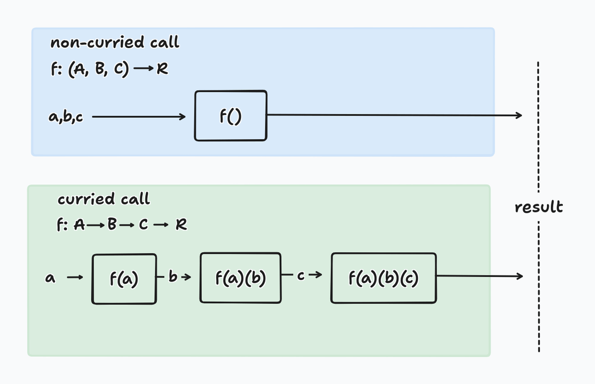
Currying is the observation that a function of two arguments is the same thing as a function that takes the first argument and returns a function of the second:

Here $C^S$ means “functions from $S$ to $C$”. Going from left to right is called currying, going back is uncurrying. In category theory language, this says the functor $- \times S$ is left adjoint to the functor $(-)^S$. Keep that word, adjoint, in the back of your mind; it’s coming back.

Now, a stateful computation is one that reads some state $s \in S$, produces a result, and produces a new state. As a pure function:

Look at the shape of that: it’s $(- \times S)$ followed by $(-)^S$. It is literally the two halves of the currying adjunction glued together. That is not a coincidence, and it’s my favourite fact in this whole topic: every adjunction gives you a monad, and the State monad is the one that currying gives you.

For State, $\eta$ returns a value without touching the state:

and chaining runs the first computation, takes the result and the new state, and hands both to the next one. You get the feeling of mutable state while everything stays a pure function.

The mathematics

Definition

Let $\mathcal{C}$ be a category; for programmers, think of it as “types and functions”. A monad on $\mathcal{C}$ is a triple $(T, \eta, \mu)$ where

• $T : \mathcal{C} \to \mathcal{C}$ is a functor (it sends a type $A$ to $T A$, and a function $f : A \to B$ to $Tf : TA \to TB$; this is map),
• $\eta : \text{Id} \Rightarrow T$ is a natural transformation called the unit, with components $\eta_A : A \to TA$,
• $\mu : T^2 \Rightarrow T$ is a natural transformation called the multiplication, with components $\mu_A : TTA \to TA$ (this is flatten or join).

They have to satisfy three laws. Associativity:

and the two unit laws:

Read them in words. Associativity says that if you have three layers of context, it doesn’t matter whether you flatten the inner two first or the outer two first. The unit laws say that wrapping something in a trivial layer and then flattening gives you back what you started with, whichever side you add the layer on.

If those look like the laws of a monoid ($(xy)z = x(yz)$ and $1x = x = x1$), that’s because they are. A monad is a monoid where the elements are functors, “multiplication” is composition of functors, and the unit is the identity functor. Hence the infamous line: a monad is just a monoid in the category of endofunctors. It sounds like a joke, but it’s actually a correct and fairly compact definition.

Checking against Maybe: $\mu$ takes $\text{Maybe}(\text{Maybe}\,A) = (A + 1) + 1$ and collapses it to $A + 1$ by sending $\text{just}(\text{just}(a))$ to $\text{just}(a)$ and both kinds of $\text{nothing}$ to $\text{nothing}$. You can check the laws by hand in a minute.

For lists: $T A$ is finite lists of $A$, $\eta(a) = [a]$, and $\mu$ concatenates a list of lists. Associativity of $\mu$ is just associativity of concatenation.

The Kleisli category

Here’s the first big idea. In programming, we rarely work with $\mu$ directly. We work with functions of the form

“functions that return a value in context”. Kleisli’s insight was that these functions form a category of their own, where the context is handled automatically.

The Kleisli category $\mathcal{C}_T$ has:

• the same objects as $\mathcal{C}$,
• a morphism $A \to B$ in $\mathcal{C}_T$ is a morphism $A \to TB$ in $\mathcal{C}$,
• the identity on $A$ is $\eta_A : A \to TA$,
• composition of $f : A \to TB$ and $g : B \to TC$ is

Read the composition right to left: run $f$ to get a $TB$; map $g$ over it to get a $TTC$; flatten with $\mu$ to get a $TC$. That’s exactly the “chain these context-returning functions” operation from the Maybe example, now stated once for every monad. People write it as $g \mathrel{<\!=\!<} f$, or $f \mathrel{>\!=\!>} g$ in the other order, and call it the fish operator.

The monad laws are exactly what make this a category. Associativity of $\mu$ gives associativity of $\circ_T$, and the unit laws make $\eta$ an identity:

This is, I think, the cleanest way to say what monads give programmers: a monad turns effectful functions into something you can compose like ordinary functions, with the same laws. That’s all. The rest is notation.

Kleisli also showed how this answers the 1965 question. There’s a functor $F_T : \mathcal{C} \to \mathcal{C}_T$ that sends a plain function $f$ to $\eta \circ f$, and a functor $U_T : \mathcal{C}_T \to \mathcal{C}$ that sends $A$ to $TA$. These are adjoint, $F_T \dashv U_T$, and the monad you get back from them is the original $T$.

Monad algebras

The second construction asks a different question. Instead of “what are the functions in context?”, it asks: what does it mean to be able to evaluate a context?

An algebra for the monad $T$ (often called a $T$-algebra) is an object $A$ together with a morphism

that collapses the context, in a way that respects the monad:

The first law says: if I wrap a value trivially and then evaluate, I get the value back. The second says: if I have two layers, I can evaluate the inner layer then the outer, or flatten first and evaluate once, and I get the same answer.

This is easiest to feel with the list monad. A list-algebra is a set $A$ with a map $a : \text{List}\,A \to A$ that turns any list of elements into a single element, consistently. Take $A = \mathbb{N}$ and $a = \text{sum}$:

Both laws hold. In fact, list-algebras are exactly monoids: give me a monoid and folding with its operation is an algebra; give me an algebra and $x \cdot y = a([x, y])$ with unit $a([\,])$ is a monoid. Similarly, Maybe-algebras are pointed sets: the algebra has to say where $\text{nothing}$ goes, and that’s just picking a default element. If you’ve ever written “value or default”, you’ve written a Maybe-algebra.

A morphism of algebras $h : (A, a) \to (B, b)$ is a function $h : A \to B$ that commutes with evaluation:

For lists, that’s a monoid homomorphism.

The Eilenberg–Moore category

The algebras and their morphisms form a category, written $\mathcal{C}^T$ and called the Eilenberg–Moore category. Like Kleisli’s, it comes with an adjunction:

$U^T$ forgets the algebra structure. $F^T$ sends $A$ to the free algebra on $A$, which is $TA$ evaluated by flattening. For lists, the free algebra on $A$ is the free monoid on $A$, which is just lists of $A$ under concatenation. Again $F^T \dashv U^T$, and again the monad you get back is $T$.

So we have two adjunctions that both produce $T$, and here is the beautiful part. Among all adjunctions that give rise to $T$, Kleisli’s is the smallest (it’s the initial one) and Eilenberg–Moore’s is the largest (it’s the terminal one). Every other adjunction producing $T$ sits between them. And the Kleisli category sits inside the Eilenberg–Moore one: it’s equivalent to the full subcategory of free algebras.

The way I think about it:

• the Kleisli category is about computations: arrows $A \to TB$, things that produce effects,
• the Eilenberg–Moore category is about handlers: maps $TA \to A$, things that consume effects and give you a plain answer.

That split is exactly how modern effect systems and algebraic effects are designed: a program is a Kleisli arrow, a handler is an algebra. Fifty-year-old mathematics, sitting quietly underneath.

Bind

Now back to code. Programmers rarely write $\mu$ or Kleisli composition directly. They write bind, usually spelled $\gg\!=$:

Notice the currying again: bind takes a wrapped value and gives back a function that wants a continuation $f$. It says: here’s a value in context, and here’s what to do with the plain value once you have it; you figure out the context.

Bind, $\mu$ and Kleisli composition are all interdefinable, so a monad can be given by any of them. From bind you recover the others:

And the monad laws, rewritten in terms of bind, become the three laws you’ll see in every Haskell tutorial:

They’re the same laws as before, just seen from the point of view of someone writing a pipeline. Left and right identity say $\eta$ doesn’t do anything. Associativity says that how you group the steps of a pipeline doesn’t matter, which is what lets you refactor a long chain into helper functions without changing its meaning.

Bind in TypeScript

TypeScript doesn’t have higher-kinded types, so we can’t write one generic Monad interface the way Haskell does. That’s fine. Writing a couple of concrete monads by hand is more illuminating anyway.

Here’s Maybe:

type Maybe<A> = { kind: 'just'; value: A } | { kind: 'nothing' }

const just = <A>(value: A): Maybe<A> => ({ kind: 'just', value })
const nothing: Maybe<never> = { kind: 'nothing' }

// η
const pure = just

// >>=
const bind = <A, B>(m: Maybe<A>, f: (a: A) => Maybe<B>): Maybe<B> =>
  m.kind === 'nothing' ? m : f(m.value)

That’s the entire monad. Now some functions that can fail:

const parseNumber = (s: string): Maybe<number> => {
  const n = Number(s)
  return Number.isNaN(n) ? nothing : just(n)
}

const reciprocal = (n: number): Maybe<number> =>
  n === 0 ? nothing : just(1 / n)

const safeSqrt = (n: number): Maybe<number> =>
  n < 0 ? nothing : just(Math.sqrt(n))

And chaining them:

const compute = (input: string): Maybe<number> =>
  bind(bind(parseNumber(input), reciprocal), safeSqrt)

compute('4')    // just(0.5)
compute('0')    // nothing   (division by zero)
compute('-4')   // nothing   (negative square root)
compute('hey')  // nothing   (not a number)

No null checks in the pipeline. Each function only deals with its own failure case, and bind handles the plumbing. If you’ve used optional chaining, or the then method on promises, you’ve been using something monad-shaped already. (Promises aren’t a lawful monad, because they flatten nested promises automatically, but they’re close enough that the intuition carries over.)

Here’s State, which is where the currying story pays off:

type State<S, A> = (s: S) => [A, S]

const pureS = <S, A>(a: A): State<S, A> => (s) => [a, s]

const bindS =
  <S, A, B>(m: State<S, A>, f: (a: A) => State<S, B>): State<S, B> =>
  (s) => {
    const [a, s1] = m(s)
    return f(a)(s1)
  }

const get = <S>(): State<S, S> => (s) => [s, s]
const put = <S>(s: S): State<S, void> => () => [undefined, s]

A tiny example: generating fresh variable names, the way a compiler would.

const fresh: State<number, string> = bindS(get<number>(), (n) =>
  bindS(put(n + 1), () => pureS(`x${n}`)),
)

const threeNames = bindS(fresh, (a) =>
  bindS(fresh, (b) =>
    bindS(fresh, (c) => pureS<number, string[]>([a, b, c])),
  ),
)

threeNames(0) // [['x0', 'x1', 'x2'], 3]

There’s no mutable counter anywhere. Every function is pure, and the state is threaded through by bind. The nesting is a bit ugly, though, and that ugliness is exactly what Haskell’s syntax was designed to get rid of.

Monads in Haskell

In Haskell, monad is a type class, and $\eta$ and bind are its methods:

class Applicative m => Monad m where
  (>>=)  :: m a -> (a -> m b) -> m b
  return :: a -> m a
  return = pure

Compare the type of bind to the math: $TA \to (A \to TB) \to TB$. It’s the same thing, character for character. The Applicative superclass is there because every monad is also a functor (that’s $T$ acting on functions) and an applicative (which lets you combine independent computations), and Haskell asks you to provide those too.

Maybe is in the standard library, but here’s what its instance looks like:

instance Monad Maybe where
  Nothing >>= _ = Nothing
  Just a  >>= f = f a

The real treat is do-notation, which is syntactic sugar for chains of bind:

compute :: String -> Maybe Double
compute input = do
  n <- readMaybe input
  r <- reciprocal n
  safeSqrt r

The compiler turns that into

readMaybe input >>= \n -> reciprocal n >>= \r -> safeSqrt r

Each arrow in do-notation is a bind, and the rest of the block is the continuation. It reads like imperative code, but it’s a pure expression, and the monad decides what “next line” means. For Maybe, “next line” means “if we didn’t fail”. For lists, it means “for each possibility”. For State, it means “with the updated state”.

Here’s the fresh-name example again, with a State monad written from scratch:

newtype State s a = State { runState :: s -> (a, s) }

instance Functor (State s) where
  fmap f (State g) = State $ \s -> let (a, s') = g s in (f a, s')

instance Applicative (State s) where
  pure a = State $ \s -> (a, s)
  State f <*> State g = State $ \s ->
    let (h, s1) = f s
        (a, s2) = g s1
    in (h a, s2)

instance Monad (State s) where
  State g >>= f = State $ \s ->
    let (a, s') = g s
    in runState (f a) s'

get :: State s s
get = State $ \s -> (s, s)

put :: s -> State s ()
put s = State $ \_ -> ((), s)

fresh :: State Int String
fresh = do
  n <- get
  put (n + 1)
  return ("x" ++ show n)

threeNames :: State Int [String]
threeNames = do
  a <- fresh
  b <- fresh
  c <- fresh
  return [a, b, c]

-- runState threeNames 0 == (["x0","x1","x2"], 3)

Compare this to the TypeScript version. Same idea, same bind, but the nesting is gone.

And finally, the one that made Haskell take monads seriously: IO. A value of type IO a is a description of a program that, when run, interacts with the world and produces an $a$. Bind lets you sequence these descriptions without ever leaving pure code:

main :: IO ()
main = do
  putStrLn "what's your name?"
  name <- getLine
  putStrLn ("hello, " ++ name)

Conceptually, IO is the State monad where the state is the entire outside world. You can’t copy the world or go back in time with it, and the monad structure makes sure you never try.

Further Reading

1. Eric Lippert’s blog series on monad
2. Monads by Mark Seeman (this is part of his series of blogs on design patterns and category theory)
3. Jeremy Bowers’ blog on Monads